Tutorial#
This tutorial provides a walkthrough for how to prepare input files for PreVABS given a cross section design.
The design of a cross section#
Figure 23 A box-beam cross section.#
The box-beam cross section shown in Fig. 23 will be used in this tutorial. All four walls and two webs are made from composite laminates. The two webs are symmetric about a middle vertical line. They are inclined such that the upper portion of both webs are closer to each other than the lower portion. The central space enclosed by the top and bottom walls and two webs is filled with an isotropic material.
The overall shape is described using four parameters, with the following values:
The width \(w = 4\) m;
The height \(h = 2\) m;
The distance \(d = 1\) m;
The angle \(a = 100^\circ\).
The materials used in this cross section are listed in Table 34 and Table 35. The layups used in this cross section are listed in Table 36.
Name |
Density |
\(E\) |
\(\nu\) |
|---|---|---|---|
\(\mathrm{kg/m^3}\) |
\(10^3\ \mathrm{Pa}\) |
||
m0 |
1.00 |
25.00 |
0.30 |
Name |
Density |
\(E_{1}\) |
\(E_{2}\) |
\(E_{3}\) |
\(G_{12}\) |
\(G_{13}\) |
\(G_{23}\) |
\(\nu_{12}\) |
\(\nu_{13}\) |
\(\nu_{23}\) |
|---|---|---|---|---|---|---|---|---|---|---|
\(10^3\ \mathrm{kg/m^3}\) |
\(\mathrm{GPa}\) |
\(\mathrm{GPa}\) |
\(\mathrm{GPa}\) |
\(\mathrm{GPa}\) |
\(\mathrm{GPa}\) |
\(\mathrm{GPa}\) |
||||
m1 |
1.86 |
37.00 |
9.00 |
9.00 |
4.00 |
4.00 |
4.00 |
0.28 |
0.28 |
0.28 |
m2 |
1.83 |
10.30 |
10.30 |
10.30 |
8.00 |
8.00 |
8.00 |
0.30 |
0.30 |
0.30 |
Component |
Name |
Material |
Ply thickness |
Orientation |
Number of plies |
|---|---|---|---|---|---|
m |
degree |
||||
Walls |
layup_1 |
m1 |
0.02 |
45 |
1 |
m1 |
0.02 |
-45 |
1 |
||
m2 |
0.05 |
0 |
1 |
||
m1 |
0.02 |
0 |
2 |
||
Webs |
layup_2 |
m2 |
0.05 |
0 |
1 |
m1 |
0.02 |
0 |
3 |
||
m2 |
0.05 |
0 |
1 |
Steps of preparing input files#
In PreVABS, a cross section is composed of components, each of which can either be a laminate or a fill. The laminate type component is composed of segments with different layups. For a realistic cross section, there may be several different ways to decompose it, which may need different information in the input files to build the model.
Hence, the first step is to decide a way of decomposition of the cross section.
For this example, the first step is trivial. The cross section can be decomposed into three components: the walls, the webs, and the fill.
At the same time, the order of creating components should also be decided. This is done by figuring out the dependence relationships between components. For this example, the exact shape of each web depends on the shape of the walls, and the shape of the fill depends on both the webs and the walls. Then the order of creation should be: first creating the walls, then the webs, and at last the fill, as shown in Fig. 24.

Figure 24 Order of components creation.#
The next step is to prepare various input files based on all design parameters listed above. In this example, all files are in the XML format. A brief summary of these input files is listed below.
A baseline file (baselines.xml), storing definitions of geometric elements.
A material file (MaterialDB.xml), storing definitions of materials and laminae.
A layup file (layups.xml), storing definitions of layups.
A main cross section file (box.xml), storing definitions of components and other configurations of modeling and analysis.
For this tutorial, all files can have arbitrary file names and be placed at any working directory, except the material database, which must be named as MaterialDB.xml and placed at the same location as where the PreVABS executable is.
Another option is to use a local file in the working directory with an arbitrary name storing the material properties. The requirement of using this local file is to explicitly provide the material file name in the main input file. Please check Section: Other input settings.
Prepare geometric elements#
As shown in Fig. 25, seven points are used to define the shape of the cross section. Points p1 to p4 define the walls, p5 and p6 define the webs, and p0 indicates the space which should be filled with some material. The origin of the coordinate system is placed at the centroid of the rectangular. Based on the design parameters \(w\), \(h\) and \(d\), coordinates of all points are found and listed in Table 37.
Figure 25 Key points defining the shape of the cross section.#
Name |
Coordinate |
|---|---|
p0 |
(0, 0) |
p1 |
(2, 1) |
p2 |
(-2, 1) |
p3 |
(-2, -1) |
p4 |
(2, -1) |
p5 |
(1, 0) |
p6 |
(-1, 0) |
Base lines are created based on key points defined above. As shown in Fig. 26, three lines are created. Line 1 is defined by connecting the four points (p1 -> p2 -> p3 -> p4 -> p1). Line 2 and 3 are defined by a single point with an incline angle. For line 2, it is the point p5 with an angle of 100 degrees. For line 3, it is the point p6 with an angle of 80 degrees.
The direction of each base line is important. It is related with how the laminate is created for each segment, and how the local coordinate system is defined for each element.
The completed input file for geometry is shown in Listing 29.
Figure 26 Base lines defining the shape of the cross section.#
 1<baselines>
 2  <basepoints>
 3    <point name="p0">0  0</point>
 4    <point name="p1">2  1</point>
 5    <point name="p2">-2  1</point>
 6    <point name="p3">-2  -1</point>
 7    <point name="p4">2  -1</point>
 8    <point name="p5">1  0</point>
 9    <point name="p6">-1  0</point>
10  </basepoints>
11  <baseline name="line1" type="straight">
12    <points>p1,p2,p3,p4,p1</points>
13  </baseline>
14  <baseline name="line2" type="straight">
15    <point>p5</point>
16    <angle>100</angle>
17  </baseline>
18  <baseline name="line3" type="straight">
19    <point>p6</point>
20    <angle>80</angle>
21  </baseline>
22</baselines>
Prepare materials and layups#
Material data are stored in the material database. As stated above, this
file must be named as MaterialDB.xml and placed at the directory where
the PreVABS executable is. The format of this file is shown in
Listing 30. Arrangement of data
under the <elastic> element are different for different material
types, which can be isotropic, orthotropic, or anisotropic.
Another part of the file is the lamina data. A lamina is a unique combination of material and ply thickness. For this example, according to the layup table (:Table 36) given above, there are two laminae. One has material m1 and thickness 0.02, and another one has material m2 and thickness 0.05. It is the lamina, instead of the material, that will be used to define each layer of the layup.
 1<materials>
 2  <material name="m0" type="isotropic">
 3    <density>1.0</density>
 4    <elastic>
 5      <e>25.0e3</e>
 6      <nu>0.3</nu>
 7    </elastic>
 8  </material>
 9  <!-- =========================================================== -->
10  <material name="m1" type="orthotropic">
11    <density>1.86E+03</density>
12    <elastic>
13      <e1>3.70E+10</e1>
14      <e2>9.00E+09</e2>
15      <e3>9.00E+09</e3>
16      <g12>4.00E+09</g12>
17      <g13>4.00E+09</g13>
18      <g23>4.00E+09</g23>
19      <nu12>0.28</nu12>
20      <nu13>0.28</nu13>
21      <nu23>0.28</nu23>
22    </elastic>
23  </material>
24  <lamina name="la_m1_002">
25    <material>m1</material>
26    <thickness>0.02</thickness>
27  </lamina>
28  <!-- =========================================================== -->
29  <material name="m2" type="orthotropic">
30    <density>1.83E+03</density>
31    <elastic>
32      <e1>1.03E+10</e1>
33      <e2>1.03E+10</e2>
34      <e3>1.03E+10</e3>
35      <g12>8.00E+09</g12>
36      <g13>8.00E+09</g13>
37      <g23>8.00E+09</g23>
38      <nu12>0.30</nu12>
39      <nu13>0.30</nu13>
40      <nu23>0.30</nu23>
41    </elastic>
42  </material>
43  <lamina name="la_m2_005">
44    <material>m2</material>
45    <thickness>0.05</thickness>
46  </lamina>
47</materials>
Layup information is stored in a separate file. Based on the layup table,
the input file can be prepared with the format shown in
Listing 31. The order of the layers
defines the laying sequence from the base line. The number in the <layer>
element stands for the orientation. If there is a colon, then the number
behind it stands for the number of plies in this layer. If there is no
number at all, then by default this layer has only one ply with orientation
of 0 degree.
 1<layups>
 2  <layup name="layup1">
 3    <layer lamina="la_m1_002">45</layer>
 4    <layer lamina="la_m1_002">-45</layer>
 5    <layer lamina="la_m2_005">0</layer>
 6    <layer lamina="la_m1_002">0:2</layer>
 7  </layup>
 8  <layup name="layup2">
 9    <layer lamina="la_m2_005"></layer>
10    <layer lamina="la_m1_002">0:3</layer>
11    <layer lamina="la_m2_005"></layer>
12  </layup>
13</layups>
Create components#
There are two types of components in PreVABS, laminate and fill. For this example, based on the decomposition we did at the begining of this section, there are three laminate-type components and one fill-type component. Besides, the sequence of creating components is important as stated at the beginning of this section. This is defined by declaring which components are needed before creating the current one.
Each laminate-type component is composed of one or more segments. Each
segment is a unique combination of a base line and a layup. The layup
can be created on either side of the base line. This is controlled by
an attribute direction, which can be either left or right. This can
be understood as the left- or right-hand side when walking along the
base line, as shown in Fig. 27.
As for the ordering, the walls should be completed first, since its inner boundary is needed to trim the base lines of both webs. Hence, each web component depends on the walls component, as shown in Listing 32.
Figure 27 Layup directions for each segment.#
 1<component name="walls">
 2  <segment>
 3    <baseline>line1</baseline>
 4    <layup>layup1</layup>
 5  </segment>
 6</component>
 7<component name="web1" depend="walls">
 8  <segment>
 9    <baseline>line2</baseline>
10    <layup>layup2</layup>
11  </segment>
12</component>
13<component name="web2" depend="walls">
14  <segment>
15    <baseline>line3</baseline>
16    <layup direction="right">layup2</layup>
17  </segment>
18</component>
The fill-type component is defined by a point and a material. Here, the point p0 is used to indicate that the material should be filled in the space in the middle enclosed by the walls and both webs. At the same time, the dependent components are also decided, as shown in Listing 33.
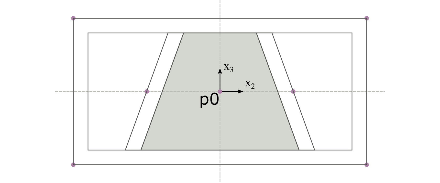
Figure 28 The fill-type component.#
1<component name="fill" type="fill" depend="walls,web1,web2">
2  <location>p0</location>
3  <material>m0</material>
4</component>
Set other configurations and complete the main input file#
Besides the definitions of components, the main input file of the cross section contains several other required or optional settings.
The first part is the <include> settings, which is required. This
contains names of the base lines and layups files.
The second part is the <analysis> settings, which is optional.
This contains configurations used by VABS for the cross-sectional analysis.
For this example, the <model> setting is set to 1, which means that
the Timoshenko beam model will be used and the 6x6 stiffness matrix will
be calculated.
The last part is the <general> settings, which is optional. This
part contains global configurations for the shape and meshing of the
cross section. Here, the global mesh size is set to 0.02.
The completed main input file for the cross section is shown in Listing 34.
 1<cross_section name="box">
 2  <include>
 3    <baseline>baselines</baseline>
 4    <layup>layups</layup>
 5  </include>
 6  <analysis>
 7    <model>1</model>
 8  </analysis>
 9  <general>
10    <mesh_size>0.02</mesh_size>
11  </general>
12  <component name="walls">
13    <segment>
14      <baseline>line1</baseline>
15      <layup>layup1</layup>
16    </segment>
17  </component>
18  <component name="web1" depend="walls">
19    <segment>
20      <baseline>line2</baseline>
21      <layup>layup2</layup>
22    </segment>
23  </component>
24  <component name="web2" depend="walls">
25    <segment>
26      <baseline>line3</baseline>
27      <layup direction="right">layup2</layup>
28    </segment>
29  </component>
30  <component name="fill" type="fill" depend="walls,web1,web2">
31    <location>p0</location>
32    <material>m0</material>
33  </component>
34</cross_section>
Execution and results#
Once all input files are prepared, the cross section can be created and homogenized using the following command:
prevabs -i box.xml -h -v -e
If everything works successfully, Gmsh will be called and the cross section
will be plotted as shown in Fig. 29
(the display of element edges is turned off in the figure for clarity),
and VABS homogenization analysis will be carried out and effective beam
properties can be found in the file box.sg.K. The effective Timoshenko
stiffness matrix is listed in Table 38.
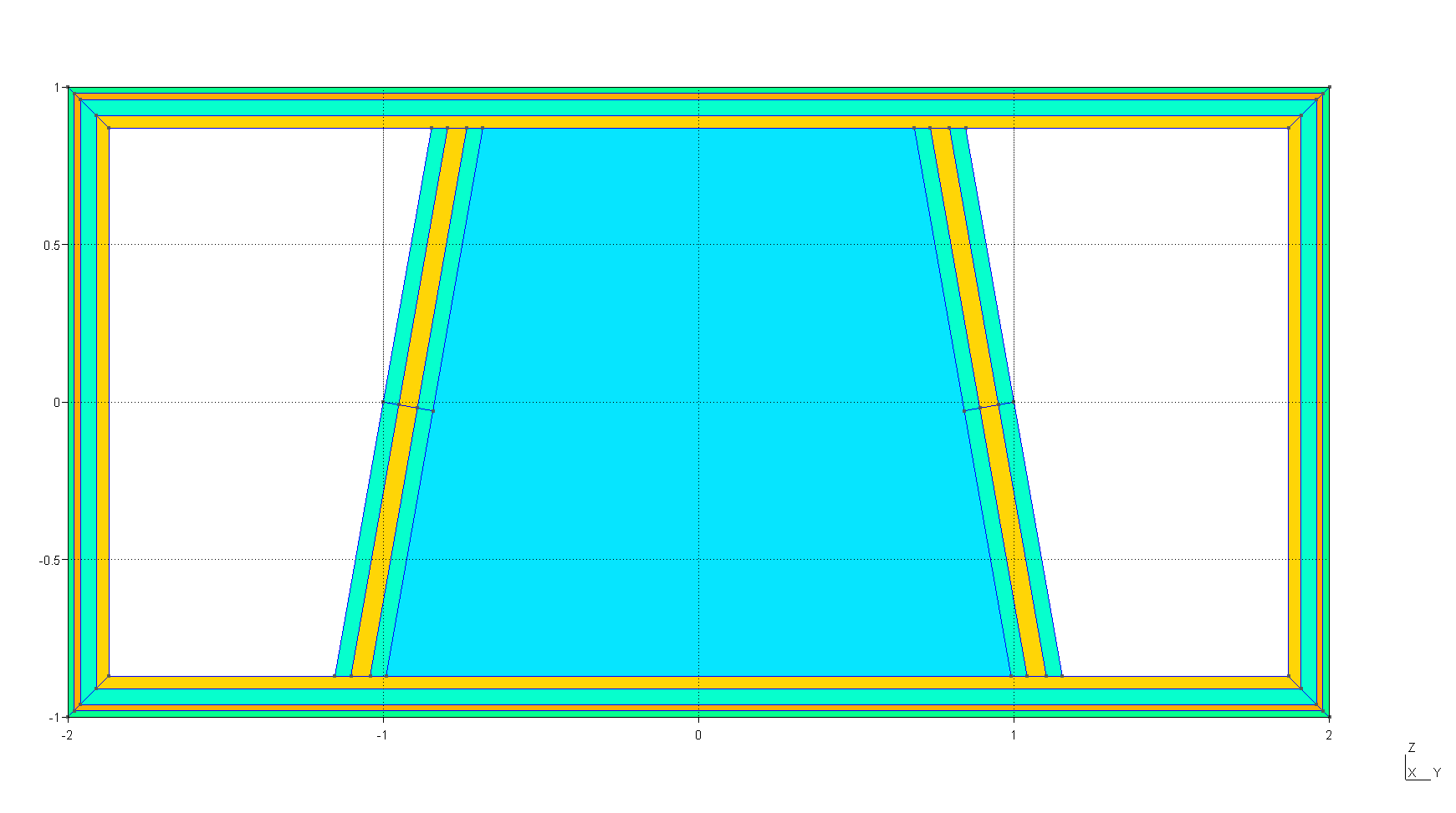
Figure 29 The cross section created by PreVABS and plotted by Gmsh.#
3.991E+10 |
-1.662E+05 |
-4.037E+01 |
4.204E+07 |
-4.358E+03 |
2.867E+01 |
-1.662E+05 |
6.743E+09 |
3.945E+04 |
-2.918E+08 |
-1.577E+07 |
-4.150E+03 |
-4.037E+01 |
3.945E+04 |
6.165E+09 |
8.220E+03 |
-2.897E+03 |
-8.700E+06 |
4.204E+07 |
-2.918E+08 |
8.220E+03 |
1.972E+10 |
2.721E+05 |
3.303E+02 |
-4.358E+03 |
-1.577E+07 |
-2.897E+03 |
2.721E+05 |
2.173E+10 |
-3.025E+04 |
2.867E+01 |
-4.150E+03 |
-8.700E+06 |
3.303E+02 |
-3.025E+04 |
6.728E+10 |