Single objective optimization of multiple cross-sections to match target beam properties

Problem description

The goal of this problem is to design a composite rotor blade for some desired beam properties, which could be given from an old design or requirements from rotor simulations.

The target beam properties are listed in the table below.

Table 23 Target beam properties

\(r/R\)	\(GJ\)	\(EI_f\)	\(EI_c\)
	\(\mathrm{lb \cdot ft}\)	\(\mathrm{lb \cdot ft}\)	\(\mathrm{lb \cdot ft}\)
0.2	0.17976e6	0.19162e6	0.32572e7
0.3	0.16882e6	0.15417e6	0.59786e7
0.4	0.16882e6	0.15417e6	0.57986e7
0.5	0.17058e6	0.16042e6	0.58384e7
0.6	0.17208e6	0.16042e6	0.58396e7
0.7	0.17208e6	0.16319e6	0.48434e7
0.8	0.13337e6	0.12709e6	0.37748e7
0.9	0.47441e6	0.38724e6	0.91526e7
0.9371	0.66027e6	0.53895e6	0.12738e8
1	22757	6927.3	0.41657e6

Parameterization

As illustrated in the previous section, parameters should be identified first at the two levels. At the cross-sectional level, consider a box-spar type structure as the design concept or topology, as shown in Fig. 8 and Fig. 9. Fig. 8 shows the parameters controlling the shape and size of components, such as locations of spar webs, and location and size of the non-structural mass. Fig. 9 shows the parameters controlling the layup scheme of box spar, front and back laminates, including material selection, fiber angle, and number of plies.

Figure 8 Shape parameters.

Figure 9 Material parameters.

At the blade level, distribution functions of cross-sectional parameters are defined. In this study, three types of distributions are considered: constant, linear interpolation, and step interpolation. A summary of cross-sectional parameters and corresponding distribution functions are given in Table 24.

Table 24 Summary of blade level distributions of cross-sectional parameters.

Cross-sectional parameter	Blade level distribution	Description
\(a^{wl}_2\)	Linear interpolation of six pairs of \((\bar{r}, \bar{a}^{wl}_2)\)	Location of the front (leading) spar web
\(a^{wt}_2\)	Linear interpolation of six pairs of \((\bar{r}, \bar{a}^{wt}_2)\)	Location of the back (trailing) spar web
\(a^{nsm}_2\)	Linear interpolation of six pairs of \((\bar{r}, \bar{a}^{nsm}_2)\)	Location of the non-structural mass center
\(r^{nsm}\)	Constant function \(\bar{r}^{nsm}\)	Radius of the non-structural mass
\(\theta^s_1,\theta^s_2,\theta^s_3,\theta^s_4\)	Step interpolation of five pairs of \((\bar{r}, \bar{\theta}^s_i)\)	Fiber angle of layer \(i\) of the box spar layup
\(n^s\)	Step interpolation of five pairs of \((\bar{r}, \bar{n}^s_i)\)	Number of plies of each layer of the box spar layup
\(\theta^f,\theta^b\)	Constant function of \(\bar{\theta}^f\) and \(\bar{\theta}^b\)	Fiber angle of each layer of the front and back layups
\(n^f,n^b\)	Constant function of \(\bar{n}^f\) and \(\bar{n}^b\)	Number of plies of each layer of the front and back layups
\(l^s, l^f, l^b\)	Constant function of \(\bar{l}^s\), \(\bar{l}^f\) and \(\bar{l}^b\)	Lamina choice of each layer of the box spar, front, and back layups

More details on the parameterization can be found in the section Parameterization of Composite Slender Structures.

Optimization setup

Design variables

The coefficients controlling the distribution functions listed in Table 24 are the true design variables in the optimization. A summary of design variables is given in Table 25.

Table 25 Design variables

Design variable	Symbol in optimization	Type	Range	Description
\((\bar{a}^{wl}_2)_1,\dots,(\bar{a}^{wl}_2)_6\)	\(x_1,\dots,x_6\)	Continuous	[0.8, 0.9]	Coefficients of the interpolation function for the leading spar web location \(a^{wl}_2\) (non-dimensional)
\((\bar{a}^{wt}_2)_1,\dots,(\bar{a}^{wt}_2)_6\)	\(x_{7},\dots,x_{12}\)	Continuous	[0.5, 0.7]	Coefficients of the interpolation function for the trailing spar web location \(a^{wt}_2\) (non-dimensional)
\((\bar{a}^{nsm}_2)_1,\dots,(\bar{a}^{nsm}_2)_6\)	\(x_{13},\dots,x_{18}\)	Continuous	[0.95, 0.985]	Coefficients of the interpolation function for the non-structural mass center location \(a^{nsm}_2\) (non-dimensional)
\(\bar{r}^{nsm}\)	\(x_{19}\)	Continuous	[0.001, 0.01]	Radius of the non-structural mass for the whole blade (non-dimensional)
\((\bar{\theta}^{s}_1)_1,\dots,(\bar{\theta}^{s}_1)_5\)	\(x_{20},\dots,x_{24}\)	Discrete	[-89, 90]	Coefficients of the interpolation function for fiber angle of layer 1 of the spar layup \(\theta^{s}_1\)
\((\bar{\theta}^{s}_2)_1,\dots,(\bar{\theta}^{s}_2)_5\)	\(x_{25},\dots,x_{29}\)	Discrete	[-89, 90]	Coefficients of the interpolation function for fiber angle of layer 2 of the spar layup \(\theta^{s}_2\)
\((\bar{\theta}^{s}_3)_1,\dots,(\bar{\theta}^{s}_3)_5\)	\(x_{30},\dots,x_{34}\)	Discrete	[-89, 90]	Coefficients of the interpolation function for fiber angle of layer 3 of the spar layup \(\theta^{s}_3\)
\((\bar{\theta}^{s}_4)_1,\dots,(\bar{\theta}^{s}_4)_5\)	\(x_{35},\dots,x_{39}\)	Discrete	[-89, 90]	Coefficients of the interpolation function for fiber angle of layer 4 of the spar layup \(\theta^{s}_4\)
\((\bar{n}^{s})_1,\dots,(\bar{n}^{s})_5\)	\(x_{40},\dots,x_{44}\)	Discrete	[1, 20]	Coefficients of the interpolation function for number of plies of the spar layup \(n^{s}\)
\(\bar{\theta}^{f}\)	\(x_{45}\)	Discrete	[-89, 90]	Fiber angle of the front (leading) layup \(\theta^{f}\)
\(\bar{\theta}^{b}\)	\(x_{46}\)	Discrete	[-89, 90]	Fiber angle of the back (trailing) layup \(\theta^{b}\)
\(\bar{n}^{f}\)	\(x_{47}\)	Discrete	[1, 20]	Number of plies of the front (leading) layup \(n^{f}\)
\(\bar{n}^{b}\)	\(x_{48}\)	Discrete	[1, 20]	Number of plies of the back (trailing) layup \(n^{b}\)
\(\bar{l}^{s}\)	\(x_{49}\)	Discrete	[1, 4]	Lamina choice of the spar layup \(l^{s}\)
\(\bar{l}^{f}\)	\(x_{50}\)	Discrete	[1, 4]	Lamina choice of the front (leading) layup \(l^{f}\)
\(\bar{l}^{b}\)	\(x_{51}\)	Discrete	[1, 4]	Lamina choice of the back (trailing) layup \(l^{b}\)

Objective function

To match the target beam properties, this example uses the weighted sum method, i.e., to minimize the maximum absolute value among the three differences of the calculated properties from the targets:

(1)\[f(\mathbf{x}) = w_1 \left| \frac{GJ-\hat{GJ}}{\hat{GJ}} \right| + w_2 \left| \frac{EI_f-\hat{EI}_f}{\hat{EI}_f} \right| + w_3 \left| \frac{EI_c-\hat{EI}_c}{\hat{EI}_c} \right|\]

where \(\hat{(\cdot)}\) is the target value.

Constraints

No other constraints are considered in this example beside the boundary constraints of design variables.

Method

Single objective genetic algorithm (SOGA) provided by Dakota is used. The method is configured in the following way:

• Maximum number of functional evaluations: 20,000

• Size of population: 200

• Random seed: 1027

• Evaluation concurrency: 20

The rest are default values given by Dakota.

Running of the example

1. Go to {IVABS_ROOT}\examples\e1_uh60_sopt_stf.

2. Run python run.py uh60_blade.yml.

Result

Table 26 Performance of the optimization

Total number of evaluations	16873
Total running time (wall clock)	20568.8 sec (~= 5 hr 40 min)
CPU model	Intel(R) Xeon(R) Gold 6134 CPU @ 3.20GHz
CPU cores	16
Memory	95 GB

Evolution

Figure 10 Evoluation of the objective function.

Final design

Figure 11 Comparison of beam properties between the optimum design and target values.

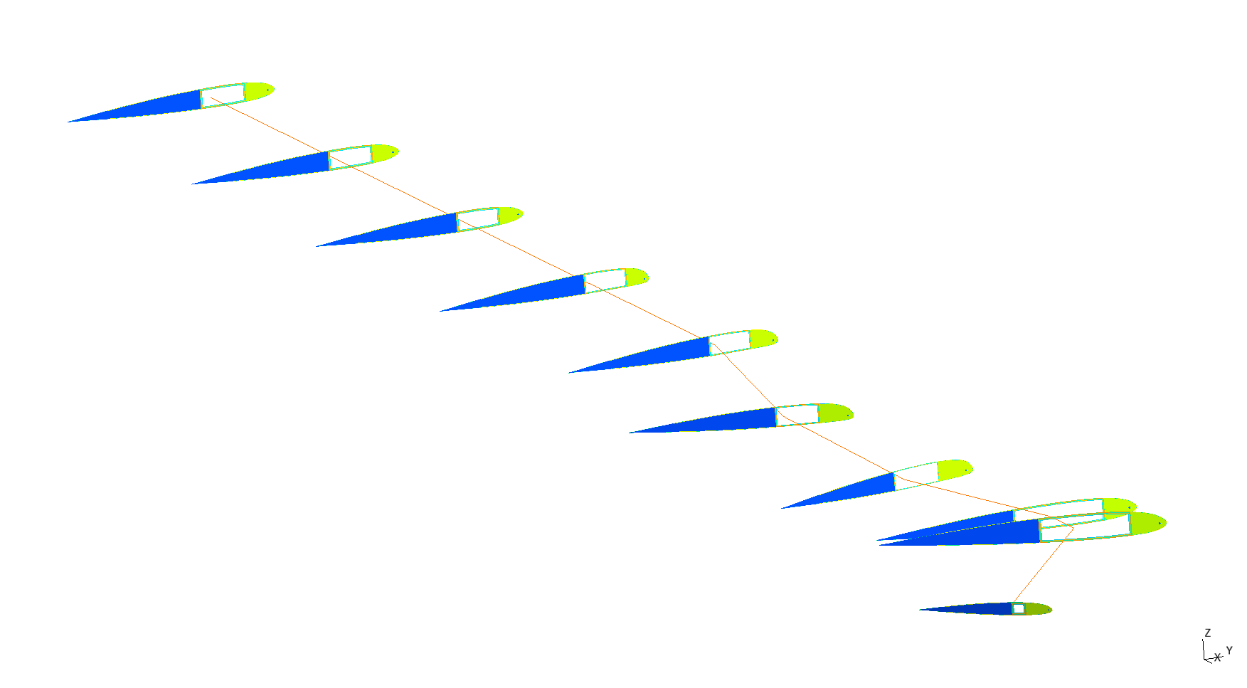
Figure 12 Plot of the ten cross-sections of the optimum design.