Visualize Abaqus Element Local Coordinate Systems#
Problem description#
An Abaqus cross-section can contain an element property reference coordinate
system (property_ref_csys) that determines the material axes. Before sending
the model to a solver, it is useful to inspect both the complete mesh and the
direction of the local y1, y2, and y3 axes.
Explaination of the solution#
plot_local_csys.py reads sg2_airfoil.inp as a 2D Abaqus structure gene and
passes its mesh to sgio.create_pyvista_plotter(). The reusable scene
factory converts the mesh, resolves each element’s local coordinate system,
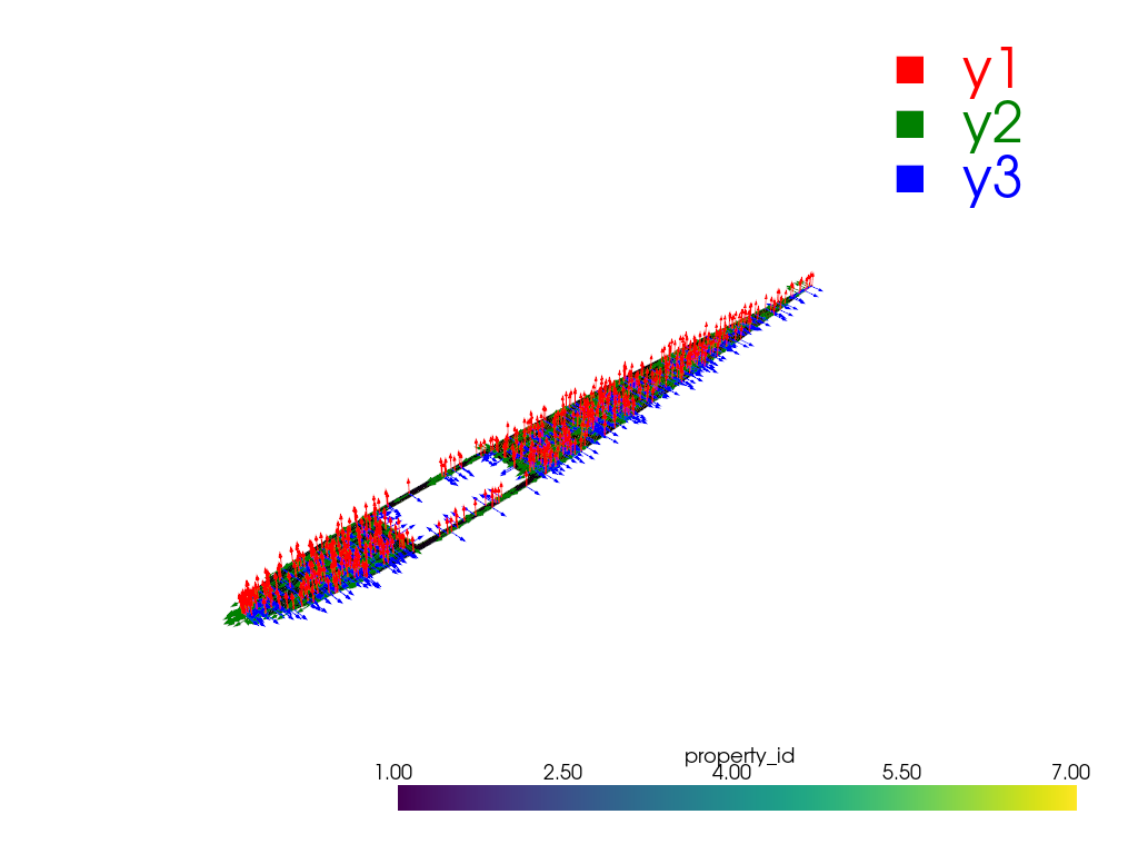
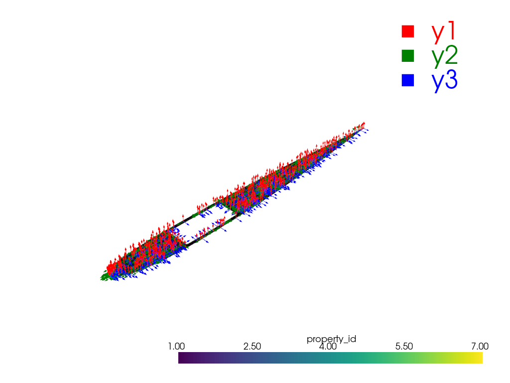
and exports a PNG scene. Red, green, and blue arrows represent
y1, y2, and y3, respectively.
The airfoil has many elements, so the script displays an evenly spaced sample
of 500 coordinate systems by default. The mesh remains complete; use
--max-axes to display more or fewer arrows.
Install PyVista once:
uv sync --extra pyvista
Run the example:
uv run python examples/convert_abaqus_cs_to_vabs/plot_local_csys.py
Result#
The script writes sg2_airfoil_local_csys.png with the local-axis arrows
overlaid.
--axis-scale is an arrow length in mesh coordinate units. If it is omitted,
the factory uses 2.5% of the mesh bounding-box diagonal.
List of all files#
plot_local_csys.py: Main script.
sg2_airfoil.inp: Abaqus input cross-section.
sg2_airfoil_local_csys.png: Generated PyVista screenshot.