Airfoil (MH-104)

Problem description

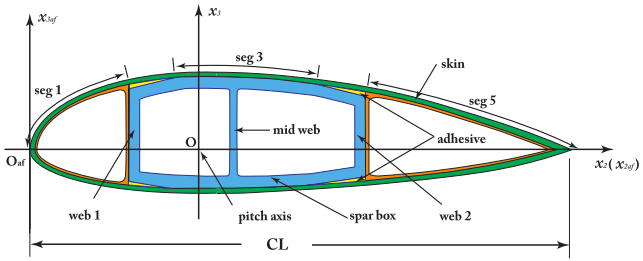
Figure 50 Sketch of a cross section for a typical wind turbine blade [CHEN2010].

This example demonstrates the capability of building a cross section having an airfoil shape, which is commonly seen on wind turbine blades or helicopter rotor blades. This example is also studied in [CHEN2010]. A sketch of a cross section for a typical wind turbine blade is shown in Fig. 50. The airfoil is MH 104 (http://m-selig.ae.illinois.edu/ads/coord_database.html#M). In this example, the chord length \(CL=1.9\) m. The origin O is set to the point at 1/4 of the chord. Twist angle \(\theta\) is \(0^\circ\). There are two webs, whose right boundaries are at the 20% and 50% location of the chord, respectively. Both low pressure and high pressure surfaces have four segments. The dividing points between segments are listed in Table 27. Materials are given in Table 28 and layups are given in Table 29. A complete \(6\times 6\) stiffness matrix is given in Table 30. Complete input files can be found in examples\ex_airfoil\, including mh104.xml, basepoints.dat, baselines.xml, materials.xml, and layups.xml.

Table 27 Dividing points

Between segments	Low pressure surface	High pressure surface
	\((x, y)\)	\((x, y)\)
1 and 2	(0.004053940, 0.011734800)	(0.006824530, -0.009881650)
2 and 3	(0.114739930, 0.074571970)	(0.126956710, -0.047620490)
3 and 4	(0.536615950, 0.070226120)	(0.542952100, -0.044437080)

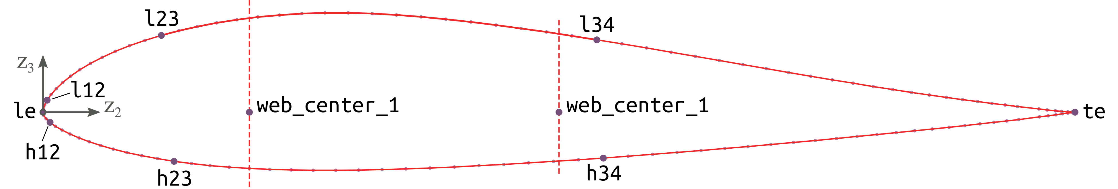
Figure 51 Base points of the tube cross section.

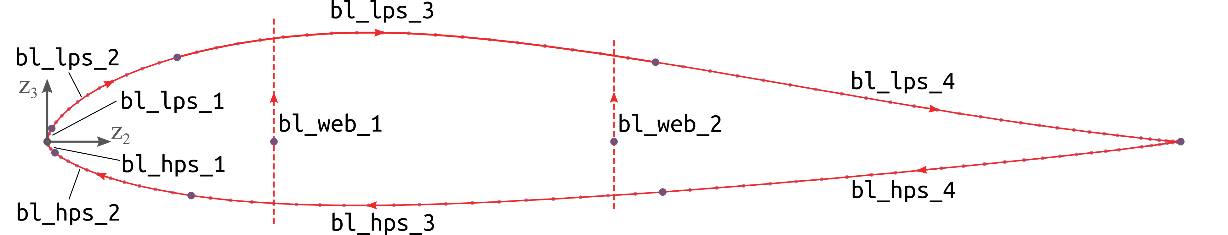
Figure 52 Base lines of the tube cross section.

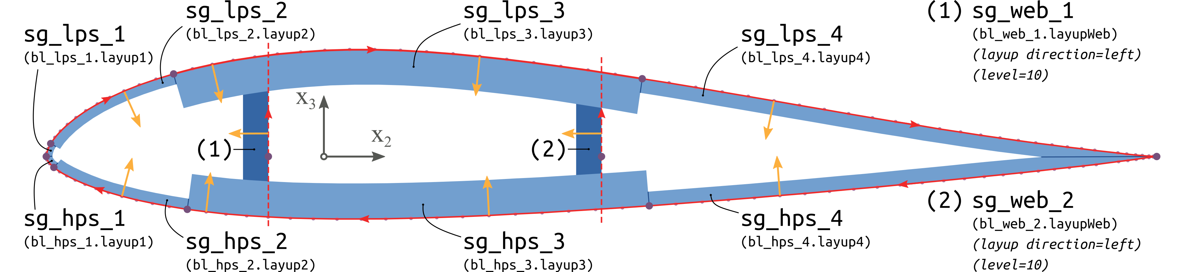
Figure 53 Segments of the tube cross section.

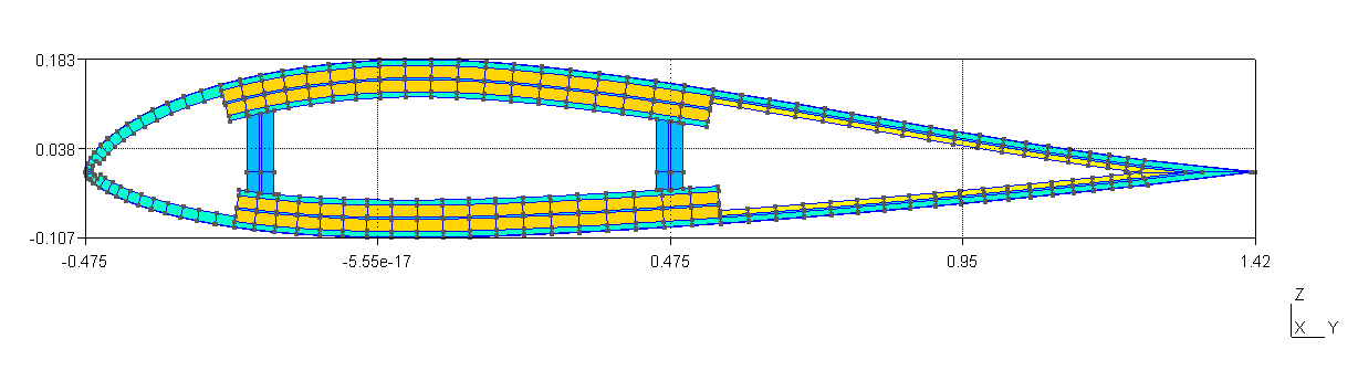
Figure 54 Meshed cross section viewed in Gmsh.

Table 28 Material properties

Name	Type	Density	\(E_{1}\)	\(E_{2}\)	\(E_{3}\)	\(G_{12}\)	\(G_{13}\)	\(G_{23}\)	\(\nu_{12}\)	\(\nu_{13}\)	\(\nu_{23}\)
		\(10^3\ \mathrm{kg/m^3}\)	\(\mathrm{GPa}\)	\(\mathrm{GPa}\)	\(\mathrm{GPa}\)	\(\mathrm{GPa}\)	\(\mathrm{GPa}\)	\(\mathrm{GPa}\)
Uni-directional FRP	orthotropic	1.86	37.00	9.00	9.00	4.00	4.00	4.00	0.28	0.28	0.28
Double-bias FRP	orthotropic	1.83	10.30	10.30	10.30	8.00	8.00	8.00	0.30	0.30	0.30
Gelcoat	orthotropic	1.83	1e-8	1e-8	1e-8	1e-9	1e-9	1e-9	0.30	0.30	0.30
Nexus	orthotropic	1.664	10.30	10.30	10.30	8.00	8.00	8.00	0.30	0.30	0.30
Balsa	orthotropic	0.128	0.01	0.01	0.01	2e-4	2e-4	2e-4	0.30	0.30	0.30

Table 29 Layups

Name	Layer	Material	Ply thickness	Orientation	Number of plies
			\(\mathrm{m}\)	\(\circ\)
layup_1	1	Gelcoat	0.000381	0	1
	2	Nexus	0.00051	0	1
	3	Double-bias FRP	0.00053	20	18
layup_2	1	Gelcoat	0.000381	0	1
	2	Nexus	0.00051	0	1
	3	Double-bias FRP	0.00053	20	33
layup_3	1	Gelcoat	0.000381	0	1
	2	Nexus	0.00051	0	1
	3	Double-bias FRP	0.00053	20	17
	4	Uni-directional FRP	0.00053	30	38
	5	Balsa	0.003125	0	1
	6	Uni-directional FRP	0.00053	30	37
	7	Double-bias FRP	0.00053	20	16
layup_4	1	Gelcoat	0.000381	0	1
	2	Nexus	0.00051	0	1
	3	Double-bias FRP	0.00053	20	17
	4	Balsa	0.003125	0	1
	5	Double-bias FRP	0.00053	0	16
layup_web	1	Uni-directional FRP	0.00053	0	38
	2	Balsa	0.003125	0	1
	3	Uni-directional FRP	0.00053	0	38

Result

Table 30 Effective Timoshenko stiffness matrix

\(\phantom{-}2.395\times 10^9\)	\(\phantom{-}1.588\times 10^6\)	\(\phantom{-}7.215\times 10^6\)	\(-3.358\times 10^7\)	\(\phantom{-}6.993\times 10^7\)	\(-5.556\times 10^8\)
\(\phantom{-}1.588\times 10^6\)	\(\phantom{-}4.307\times 10^8\)	\(-3.609\times 10^6\)	\(-1.777\times 10^7\)	\(\phantom{-}1.507\times 10^7\)	\(\phantom{-}2.652\times 10^5\)
\(\phantom{-}7.215\times 10^6\)	\(-3.609\times 10^6\)	\(\phantom{-}2.828\times 10^7\)	\(\phantom{-}8.440\times 10^5\)	\(\phantom{-}2.983\times 10^5\)	\(-5.260\times 10^6\)
\(-3.358\times 10^7\)	\(-1.777\times 10^7\)	\(\phantom{-}8.440\times 10^5\)	\(\phantom{-}2.236\times 10^7\)	\(-2.024\times 10^6\)	\(\phantom{-}2.202\times 10^6\)
\(\phantom{-}6.993\times 10^7\)	\(\phantom{-}1.507\times 10^7\)	\(\phantom{-}2.983\times 10^5\)	\(-2.024\times 10^6\)	\(\phantom{-}2.144\times 10^7\)	\(-9.137\times 10^6\)
\(-5.556\times 10^8\)	\(\phantom{-}2.652\times 10^5\)	\(-5.260\times 10^6\)	\(\phantom{-}2.202\times 10^6\)	\(-9.137\times 10^6\)	\(\phantom{-}4.823\times 10^8\)

Table 31 Results from reference [CHEN2010]

\(\phantom{-}2.389\times 10^9\)	\(\phantom{-}1.524\times 10^6\)	\(\phantom{-}6.734\times 10^6\)	\(-3.382\times 10^7\)	\(-2.627\times 10^7\)	\(-4.736\times 10^8\)
\(\phantom{-}1.524\times 10^6\)	\(\phantom{-}4.334\times 10^8\)	\(-3.741\times 10^6\)	\(-2.935\times 10^5\)	\(\phantom{-}1.527\times 10^7\)	\(\phantom{-}3.835\times 10^5\)
\(\phantom{-}6.734\times 10^6\)	\(-3.741\times 10^6\)	\(\phantom{-}2.743\times 10^7\)	\(-4.592\times 10^4\)	\(-6.869\times 10^2\)	\(-4.742\times 10^6\)
\(-3.382\times 10^7\)	\(-2.935\times 10^5\)	\(-4.592\times 10^4\)	\(\phantom{-}2.167\times 10^7\)	\(-6.279\times 10^4\)	\(\phantom{-}1.430\times 10^6\)
\(-2.627\times 10^7\)	\(\phantom{-}1.527\times 10^7\)	\(-6.869\times 10^2\)	\(-6.279\times 10^4\)	\(\phantom{-}1.970\times 10^7\)	\(\phantom{-}1.209\times 10^7\)
\(-4.736\times 10^8\)	\(\phantom{-}3.835\times 10^5\)	\(-4.742\times 10^6\)	\(\phantom{-}1.430\times 10^6\)	\(\phantom{-}1.209\times 10^7\)	\(\phantom{-}4.406\times 10^8\)

Note

The errors between the result and the reference are caused by the difference of modeling of the trailing edge. If reduce the trailing edge skin to a single thin layer, then the difference between the trailing edge shapes is minimized, and the two resulting stiffness matrices are basically the same, as shown in Fig. 55.

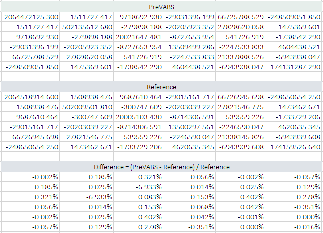
Figure 55 Comparison of stiffness matrices after modifying the trailing edge.