3.2.2. Cross-section with arbitrary shape (2D SG)#
Steps#
Step 1: Set work directory#
Menu > File > Set Work Directory…. Select the directory where you want to put all related files, .cae, .inp, .sc, etc.
Step 2: Create materials#
Create two materials, “Material-1” and “Material-2”, with arbitrary material properties.
Step 3: Create composite sections#
User can create layups using functions described in section 3.3, or using Abaqus’s own functions by hand, which is described below.
Module > Property > Create Section. Create three Solid > Composite sections, “Layup-1”, “Layup-2” and “Layup-3”, with the following configs.
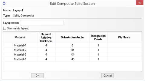
Figure 3.2.2.1 Composite section Layup-1.#

Figure 3.2.2.2 Composite section Layup-2.#
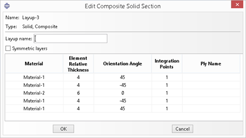
Figure 3.2.2.3 Composite section Layup-3.#
Note here that the thickness of each layer should be actual thickness instead of relative thickness.
Step 4: Draw the general shape#
According to the coordinates convention in SwiftComp, the X-axis is along the beam reference line and the cross-section is in the Y-Z plane.
Thus we need to first set our workplane to Y-Z plane.
Click Work plane  , give a New Part Name, and select 2D as the SG Dimension.
Click OK.
, give a New Part Name, and select 2D as the SG Dimension.
Click OK.
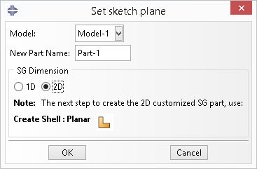
Figure 3.2.2.4 Set work plane.#
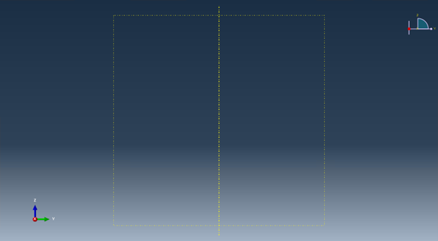
Figure 3.2.2.5 After setting the work plane.#
In Module > Part, click Create Shell: Planar, following the prompt, select the datum plane and the datum axis.
Sketch the shape shown below, with dimensions marked in the figure.
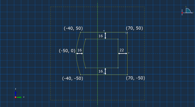
Figure 3.2.2.6 Sketch the geometry.#
Click Done, then the part will be generated.
Next we need to divide this part into four segments. Use Partition Face: Sketch to create the four segments as shown below.
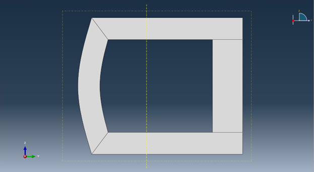
Figure 3.2.2.7 Partition the geometry.#
Step 5: Assign layups#
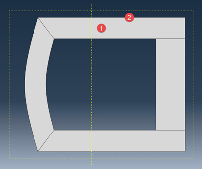
First we will assign the layup for the top segment.
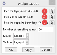
Click Assign Layups  to open the dialog box.
Pick the area 1, pick the baseline 2 and select section “Layup-1”.
Click OK.
to open the dialog box.
Pick the area 1, pick the baseline 2 and select section “Layup-1”.
Click OK.

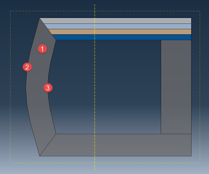
Next, assign the layup for the segment on the left. Pick the area 1, baseline 2, opposite boundary 3, give 20 sampling points and select section “Layup-1”. Click OK.
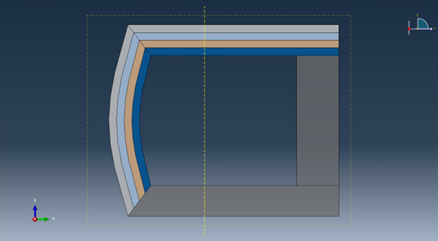
We can do the same for the rest two segments, except that we use “Layup-3” for the right segment.
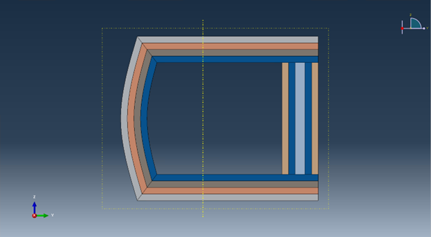
The color may change for some layers after assigning new layups. This is due to new sections created in “Layup-3”, causing the order of the section list to change, so that the color map also changes.
Step 6: Delete layups#
If users find that some layup is assigned mistakenly, it can be deleted and re-assigned.
For instance, we want to re-assign the layup for the left segment.
Click Erase Layups  .
In the dialog box pick the same baseline used for assigning the layup.
Click OK.
.
In the dialog box pick the same baseline used for assigning the layup.
Click OK.
Once done, user can assign a new layup for the empty segment. Here we assign the “Layup-2”.
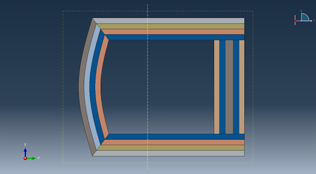
Step 7: Assign local coordinates#
In Module > Property, use Assign Material Orientation.
For a shell part in Abaqus, we can only have axis 1 and 2 in the cross-section plane. Thus we will make axis 1 and 2 as the local \(y_2\) and \(y_3\) axis in SwiftComp convention respectively. Here we will keep axis 2 (\(y_3\)) perpendicular to the outer profile edges and pointing outwards. User can also let axis 2 point inward, as long as the local orientation keeps consistency with the global coordinate and fiber orientations defined by users.
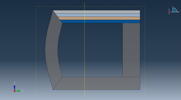
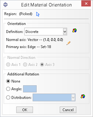
Following the prompt, we first select the top segement to be assigned a local material orientation, and click Done. Then in the prompt area, click Use Default Orientation or Other Method. In the Edit Material Orientation dialog box, select Discrete as the Orientation Definition. Then click Define… to open the Edit Discrete Orientation dialog box.
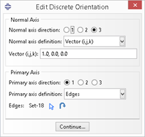
In the Normal axis definition choose Vector (i,j,k), and set the vector (1.0, 0.0, 0.0). For Primary Axis, select 1 as the Primary axis direction and Edges as the Primary axis definition. Click Edit Edges… to select the light blue edge shown in the figure below, then click Done. Use Flip Direction to make the axis pointing to the right if necessary. Click Continue… then OK to finish this assignment.
Do the same procedure for the rest three segments. Some steps may not be exactly the same. The only requirement is to make sure that the axis 2 pointing outwards.
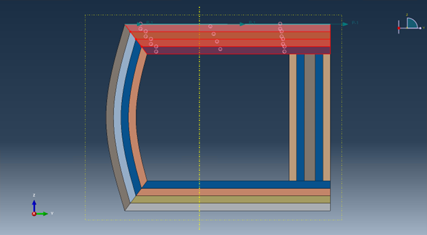
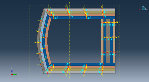
Once done, the local orientations should look like the same as the figure shown below.
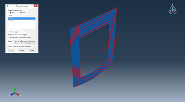
Step 8: Create assembly#
In Module > Assembly, click Create Instance and select the part created before.
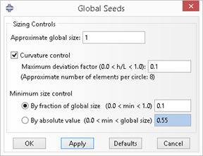
Step 9: Mesh#
In Module > Mesh, first choose Part as the Object. Then click Seed Part. In the Global Seeds dialog box, set Approximate global size to 1.
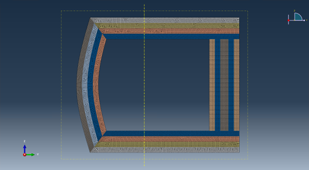
Click Mesh Part, then click Yes in the prompt area.
Step 10: Write Abaqus input file#
In Module > Job, click Create Job.
In the Create Job dialog box, set Name to “Job-1”. In the model tree, right click “Job-1”, click Write Input, then an Abaqus input file “Job-1.inp” will be created.
Step 11: Homogenization#
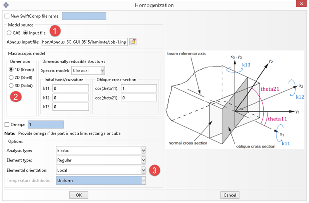
Click Homogenization button  .
In the dialog box, choose Model source > Input file.
For Abaqus input file, select the abaqus input we just created, “Job-1.inp”.
Choose Macroscopic model > Dimension > 1D (Beam).
Choose Options > Elemental orientation > Local.
Then click OK.
.
In the dialog box, choose Model source > Input file.
For Abaqus input file, select the abaqus input we just created, “Job-1.inp”.
Choose Macroscopic model > Dimension > 1D (Beam).
Choose Options > Elemental orientation > Local.
Then click OK.
Note: Since we used discrete local orientations, local coordinate systems for each element are calculated only when writing the Abaqus input file. Thus user can only choose Input file as the Model source to do the homogenization.
After a certain time, depending on the model size, SwiftComp will finish computing the cross-sectional properties and show the results in the notepad. If no error occurs, close the notepad and the process will end.
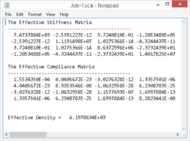
If error messages pop out, or an empty notepad file appears, please refer to the command line window for more information.