3.1.2. Square Pack Microstructure (2D SG)

2D SG preparation

In this example, assume that both fiber and matrix are isotropic materials.

Table 3.1.2.1 Material properties

Name	\(E\) GPa	\(\nu\)
Fiber	379.3	0.1
Matrix	68.3	0.3

Then click the 2D SG button then the dialog box will pop out (Fig. 2.2-3). The square pack microstructure SG has width 1.0. Set the volume fraction of fiber to 0.4. Since interphase is not needed, set the value to 0.0.

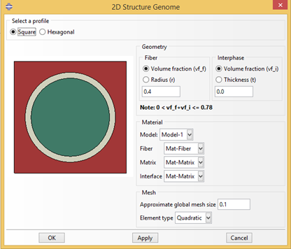
Figure 3.1.2.1 Create 2D SG dialog box.

After setting all the parameters as shown in Fig. 2.2-3, click OK to finish the creation (Fig. 2.2-4).

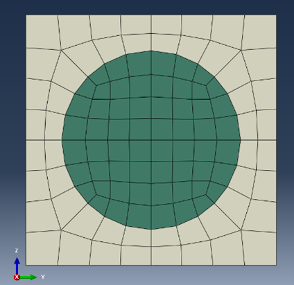
Figure 3.1.2.2 Created 2D SG.

Homogenization

Click the homogenization button then the dialog box will pop up (Fig. 2.2-6). In this example, we choose the 3D solid macro model, then the default file name will be sqrP2_nSG2_3D_S8R.sc. Click OK and wait for preparing the input file of SwiftComp and homogenization. After the computation of SwiftComp, the effective properties will pop up automatically (Fig. 2.2-7).

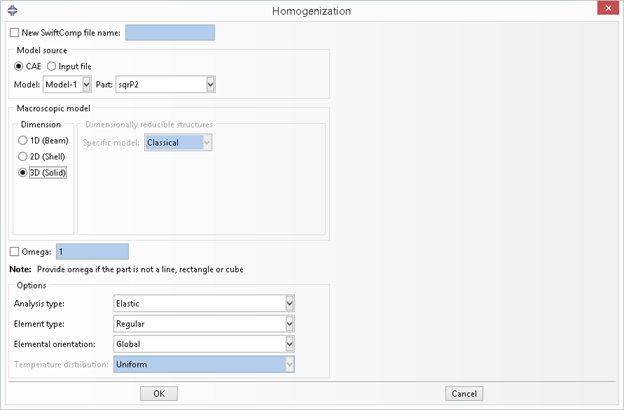
Figure 3.1.2.3 Homogenization dialog box - use 3D solid model.

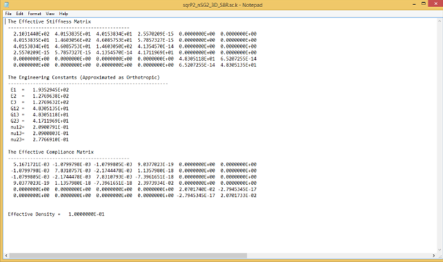
Figure 3.1.2.4 Effective properties of 3D solid model.

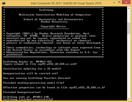
Figure 3.1.2.5 Command line window showing the SwiftComp messages.

Dehomogenization

Click the dehomogenization button then the dehomogenization dialog box will pop out (Fig. 2.2-10). We can choose the SG from CAE or choose SwiftComp input file sqrP2_nSG2_3D_S8R.sc, and then specify the required inputs as shown in Fig. 2.2-10.

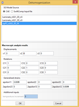
Figure 3.1.2.6 Dehomogenization parameters for 3D solid model.

Click OK and wait for SwiftComp to finish the computation. Switch to the Visualization model, the user is able to view all the field results components. In the odb tree, two sections are created, with each section containing the same material properties. The nodal stress SN11 component is shown in Fig. 2.2-11.

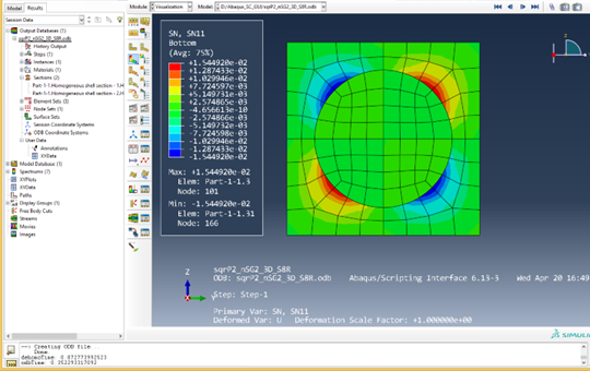
Figure 3.1.2.7 Dehomogenization results of 3D model.