3.2.1. Arbitrary Shape Inclusions Microstructure (2D SG)#
An example with user-defined microstructure is shown here, which is a rectangular SG with two arbitrarily shaped inclusions. Users can learn how to create arbitrary shapes in Abaqus-SwiftComp GUI and let SwiftComp calculate such models.
Step 1: Create materials and sections#
In this example, consider the following material properties:
Material 1: \(E\)=379.3 GPa, \(\nu\)=0.1
Material 2: \(E\)=279.3 GPa, \(\nu\)=0.1
Material 3: \(E\)=68.3 GPa, \(\nu\)=0.3
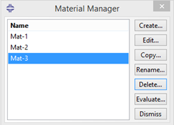
Figure 3.2.1.1 Created materials.#
Step 2: Set work plane#
Click the Work plane button  to open the dialog box.
Choose SG Dimension > 2D, then click OK.
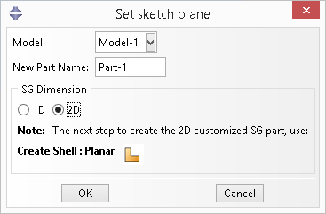
Figure 3.2.1.2 Set work plane.#
Step 3: Create geometry#
In Module > Part, click the Create Shell: Planar to sketch the geometry.
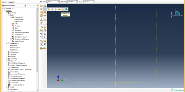
Figure 3.2.1.3 Create shell planar.#
First create the rectangular shape using points (-0.5, -1), (0.5, 1) as shown in Fig. 3.2-2(a).
Use Partition face: Sketch to create the two inclusions (Fig. 3.2-2 (b)).
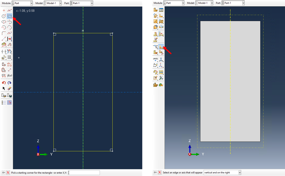
Figure 3.2.1.4 Create the overall shape of the SG.#
Create the isolated points (-0.2, 0.8), (-0.3, 0.7), (-0.3, 0.4), (-0.1, 0.6), (0, 0.8), (0, 0), (-0.1, 0), (-0.2, -0.3), (0.1, -0.5), (0.1, -0.3), and (0.2, -0.1) (see Fig. 3.2-3 (a)). Create splines through the points as shown in Fig. 3.2-3 (b).
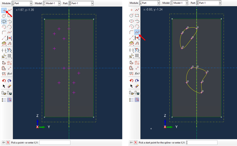
Figure 3.2.1.5 Create the inclusions of the SG.#
Step 4: Create and assign sections#
Create and assign sections as shown in Fig. 3.2-4.
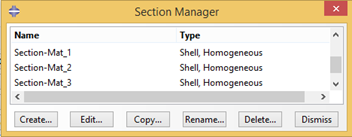
Figure 3.2.1.6 Created sections.#
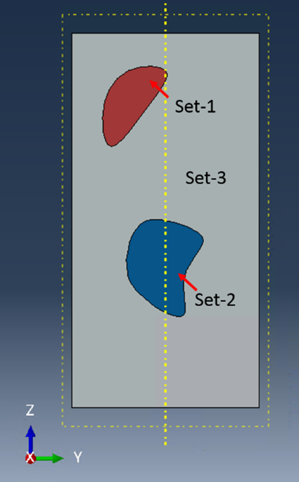
Figure 3.2.1.7 Assign sections#
Step 5: Generate mesh#
In Module > Mesh, click the Seed Part to set the mesh size. Set Approximate global size to 0.05, then click OK.
In Assign Mesh Controls, set the Element Shape to Quad-dominated, the Technique to Free, and the Algorithm to Advanced front > Use mapped meshing where appropriate.
The mesh shown in the Fig. 3.2-5 is quite irregular but can be used for homogenization analysis. However, it can be seen that there is one element (highlighted in the yellow ellipse) is abnormal. If use this mesh to do the dehomogenization, there will be an error message in the command window (Fig. 3.2-6).
Such a mesh can be repaired as shown in Fig. 3.2-7.
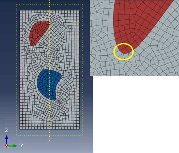
Figure 3.2.1.8 Fig. 3.2-5 Mesh need to be repaired#
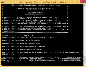
Figure 3.2.1.9 Fig. 3.2-6 Error message in dehomogenization#
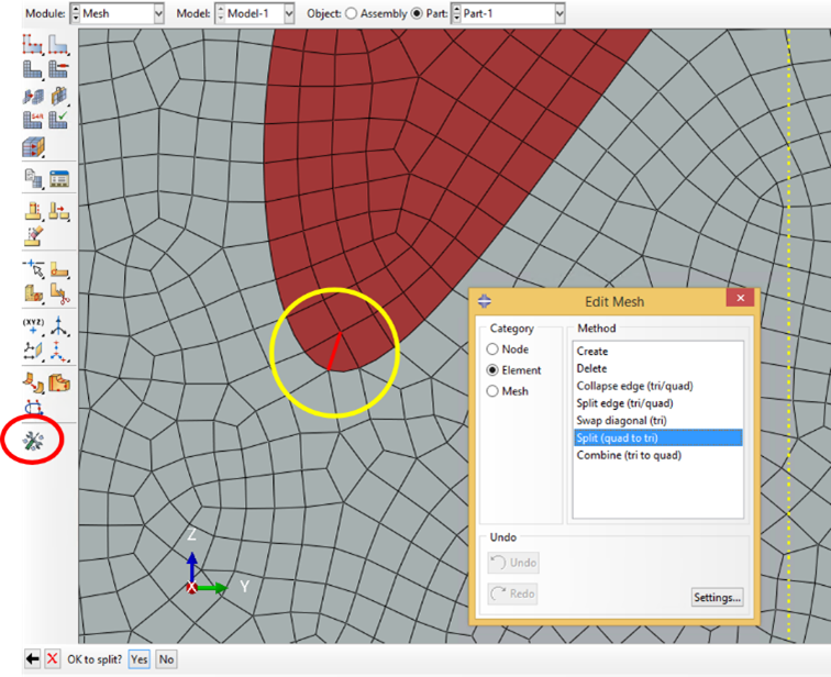
Figure 3.2.1.10 Fig. 3.2-7 repair the mesh#
Step 6: Homogenization and dehomogenization#
Click the homogenization button  then fill the dialog box as shown in the Fig. 3.2-8
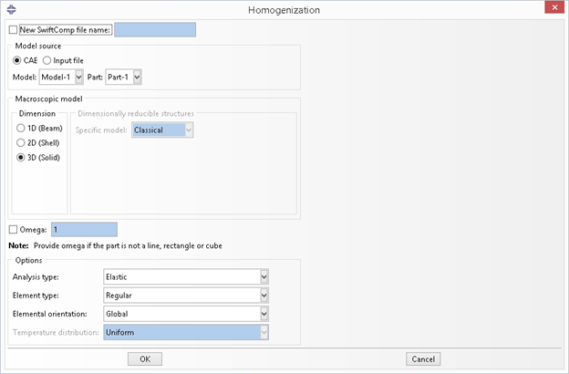
Figure 3.2.1.11 Homogenization.#
The effective properties is obtained (Fig. 3.2-9).
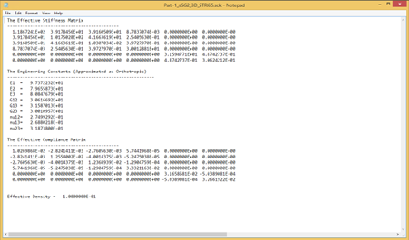
Figure 3.2.1.12 Effective properties.#
Click the dehomogenization button  then fill the dialog box as shown in the Fig. 3.2-10
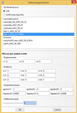
Figure 3.2.1.13 Dehomogenization.#
The local fields are obtained (Fig. 3.2-11).
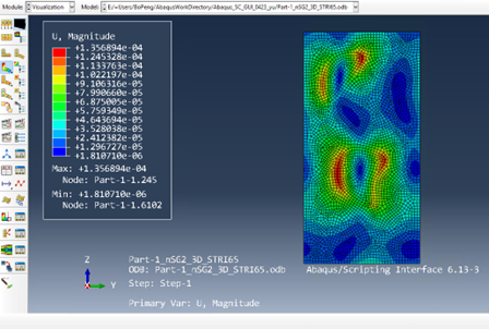
Figure 3.2.1.14 Dehomogenization result: magnitude of displacement.#