3.1.3. Spherical Inclusion Microstructure (3D SG)#
3D SG preparation#
In this example, use the following material properties:
Fiber: Young’s modulus \(E\)=379.3 GPa, Poisson’s ratio \(\nu\)=0.1
Matrix: Young’s modulus \(E\)=68.3 GPa, Poisson’s ratio \(\nu\)=0.3
Interphase: \(E_1\)=117.0 GPa, \(E_2\)=\(E_3\)=8.54 GPa, \(\nu_{12}\)=\(\nu_{13}\)=0.278, \(\nu_{23}\)=0.5, \(G_{12}\)=\(G_{13}\)=3.9 GPa, \(G_{23}\)=2.83 GPa.
Then click the 3D common SG button  then the dialog box will pop out (Fig. 2.3-3).
This 3D SG has length 1.0 in every dimension.
Set the Geometry > Inclusion > Volume fraction to 0.4.
Set the Geometry > Interphace > Volume fraction to 0.1.
then the dialog box will pop out (Fig. 2.3-3).
This 3D SG has length 1.0 in every dimension.
Set the Geometry > Inclusion > Volume fraction to 0.4.
Set the Geometry > Interphace > Volume fraction to 0.1.
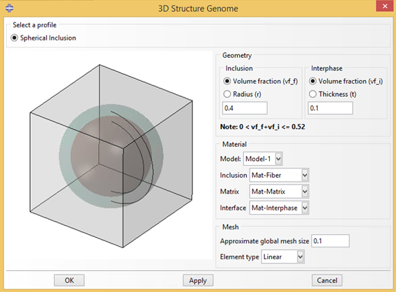
Figure 3.1.3.1 Create 3D SG dialog box.#
After setting all the parameters as shown in Fig. 2.3-3, click OK to create the SG (Fig. 2.3-4).
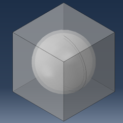
Figure 3.1.3.2 Fig. 2.3-4 The created 3D SG#
Homogenization#
Click the homogenization button  then the dialog box will pop up.
In this example, we choose the 3D solid macro model, then the default file name will be
then the dialog box will pop up.
In this example, we choose the 3D solid macro model, then the default file name will be inclusionP3_nSG3_3D_C3D4.sc.
Click OK and wait for preparing the input file of SwiftComp and homogenization.
After the computation of SwiftComp, the effective properties will pop up automatically (Fig. 2.3-6).
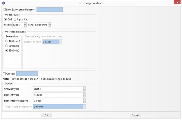
Figure 3.1.3.3 Homogenization dialog box-use 3D solid model.#
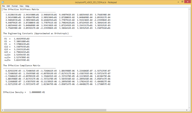
Figure 3.1.3.4 Effective properties of 3D solid model.#
Dehomogenization#
Click the dehomogenization button  then the dialog box will pop out.
Choose SG Model Source > CAE and select the model “inclusionP3_nSG3_3D_C3D4”.
Input Macroscopic analysis results as shown in Fig. 2.3-8.
then the dialog box will pop out.
Choose SG Model Source > CAE and select the model “inclusionP3_nSG3_3D_C3D4”.
Input Macroscopic analysis results as shown in Fig. 2.3-8.
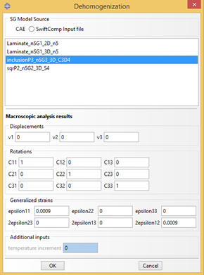
Figure 3.1.3.5 Dehomogenization parameters for 3D solid model.#
Click OK and wait for SwiftComp to finish the computation. Switch to the Visualization module, the user is able to view all the field results. In the odb tree, three sections are created, with each section containing the same material properties.
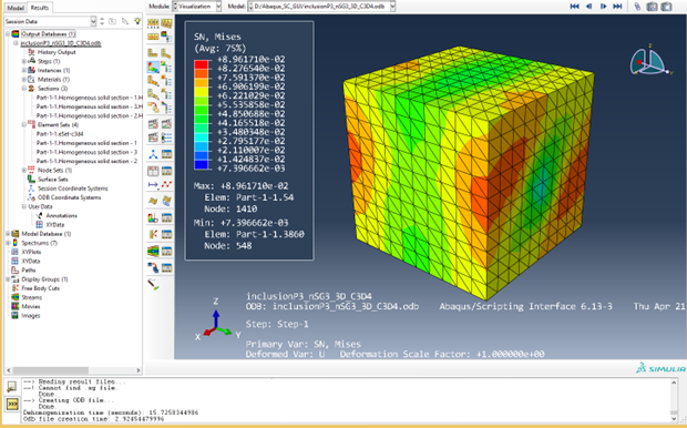
Figure 3.1.3.6 Dehomogenization results of 3D model.#