Many Builders, One Pipeline
Homogenization and anisotropy of microstructures from four modeling tools
Overview
Microstructures can be built by different tools: Dedicated tools like TexGen or microgen, or general ones like Gmsh or Abaqus/CAE (see Links for all tools). Their outputs differ in format, element types and the way material orientations are stored. This example takes one microstructure from each of four tools and runs all of them through one pipeline built on two core tools:
SwiftComp homogenizes a heterogeneous material: from a finite-element model of its Structure Gene (SG), the smallest building block of the microstructure (here a 2D cross-section or a 3D unit cell), it computes the effective properties.
sgio connects SwiftComp to the rest of the toolchain: it converts each modeling tool’s output into a SwiftComp SG input, runs SwiftComp, and reads the results back into Python.
The pipeline has three stages:
The modeling tools differ, but after sgio the pipeline is identical: only the input format and the SG dimension change from one model to the next. The effective stiffness of each model is then compared using a measure of elastic anisotropy, which puts a honeycomb, a fibre composite, a TPMS lattice and a woven fabric on one scale.
Preprocess: four builders
Each model has one geometry parameter varied over a range and two sets of constituent materials, material set 1 and material set 2. The value in bold is the representative one used for the model images and the directional Young’s modulus surfaces.
| Model | Builder | SG | Geometry parameter (representative) | Material set 1 | Material set 2 |
|---|---|---|---|---|---|
| Hexagonal honeycomb | Abaqus/CAE | 2D | wall thickness : 0.05, 0.10, 0.15, 0.20 | aluminium 5052 | AS4/8773 lamina walls, fibres along the wall |
| UD fibre composite, random fibres | Gmsh (GmshModel) | 2D | fibre count 4, 8, 12, 16 ( 0.13 to 0.50) | E-glass / epoxy | T300 carbon / epoxy |
| Schwarz-P TPMS sheet | microgen | 3D | level-set offset 0.5, 0.8, 1.1, 1.4 (solid fraction 0.14 to 0.40) | PEEK | Ti-6Al-4V |
| 2×2 plain weave | TexGen | 3D | yarn spacing 0.85, 1.0, 1.2, 1.4 | E-glass yarns / epoxy | AS4/8773 yarns / epoxy |
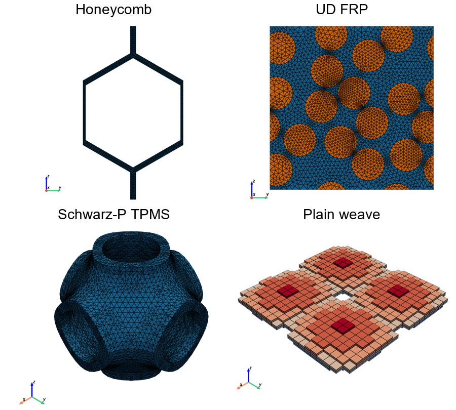
Figure 1:Representative SGs as SwiftComp receives them (read back from the .sg files), material set 1.
Honeycomb ; UD composite with 16 random fibres (); TPMS sheet at offset
0.5 (solid fraction 0.14); plain weave with the matrix voxels hidden and the yarn voxels colored
by height. The triad shows the SG axes , , ; for the 2D SGs points out of the page.
The material constants are in data/materials.json.
The four tools hand over their models in two file types:
Abaqus input decks (
.inp): the honeycomb from an Abaqus/CAE script and the weave from TexGen. Both carry materials, sections and per-element material orientations. The honeycomb uses a discrete orientation that aligns the local 1 axis with the nearest wall centerline; the weave stores each voxel’s yarn direction in a separate.orifile, which sgio follows from the deck’s*Distribution ... Input=line.Gmsh meshes (
.msh) for the UD composite and the TPMS. A mesh carries physical groups but no materials, so each comes with an SG manifest (.sg.json) that sets the SG dimension, the model space and the physical group → material binding.
Homogenization: sgio and SwiftComp
sgio converts every model file to a SwiftComp SG, and SwiftComp computes its effective
stiffness. Every case goes through the same two calls; only the input format (abaqus or
sg_manifest) and the SG dimension differ:
import sgio

# builder: (input format, SG dimension)
FORMATS = {
    "abaqus_honeycomb": ("abaqus", 2),
    "gmshmodel_udfrp": ("sg_manifest", 2),
    "microgen_tpms": ("sg_manifest", 3),
    "texgen_weave": ("abaqus", 3),
}

file_format, sgdim = FORMATS[builder]
sgio.convert(source, sg_file, file_format, "sc", file_version_out="2.1",
             sgdim=sgdim, model_space="xy" if sgdim == 2 else None, model_type="SD1")
sgio.run("swiftcomp", sg_file, "h", smdim=3)                    # writes <sg_file>.k
All results and figures use the SG axes, labelled , , (SwiftComp’s , , ).
For the 3D SGs these are the mesh axes.
A 2D SG lies in the – plane: model_space="xy" maps the mesh’s and onto the SG’s and , and is the fibre axis of the UD composite and the prism axis of the honeycomb.
The effective stiffness is a full 3D Cauchy-continuum stiffness (SD1) in both cases, so 2D and 3D microstructures are compared on the same footing.
Postprocess
Reading the SwiftComp results
sgio reads the homogenized properties back from the .k file:
import numpy as np
import sgio

model = sgio.read_output_model(f"{sg_file}.k", "sc", "sd1")
C = np.asarray(model.stff)   # 6x6 effective stiffness, Voigt order (11, 22, 33, 23, 13, 12)
rho = model.density # effective density is the effective stiffness in the SG axes .
is the effective densities.
Both are collected for every case in results/summary.csv.
Directional Young’s modulus
The Young’s modulus along a unit direction follows from the compliance , written as a fourth-order tensor:
Converting the Voigt compliance to divides the shear entries by 2 (one shear index) or 4 (two shear indices). Evaluating over a grid of directions and plotting gives a surface whose shape shows the anisotropy; a sphere means isotropy.
Energy-ratio-based anisotropy measure
The anisotropy of each is condensed into one number, the energy-ratio-based measure of elastic anisotropy Fang et al. (2019). Take a strain state and apply it in every orientation . The strain energy density then varies between a highest and a lowest value. The measure is the largest such ratio over all strain states, minus one:
means every strain state stores the same energy in every orientation, i.e. the material is isotropic. It becomes infinite when some deformation costs no energy in one orientation but a finite energy in another. The number depends neither on the coordinate system nor on the scale of .
Results
Anisotropy against density
All 32 cases on one chart:
Figure 2:Energy-ratio anisotropy measure against effective density for all cases (log-log). Color marks the microstructure, filled circles material set 1, open diamonds material set 2; lines connect the cases of one parameter range; larger symbols mark the representative parameter values.
Directional Young’s modulus
The surfaces below are for the representative value of each geometry parameter (bold in the table above):
Figure 3:Directional Young’s modulus surfaces for the representative parameter values, scaled by each surface’s maximum. One row per microstructure; the first column repeats its SG image, the other two columns are material sets 1 and 2. Axes , , are the SG axes, as in Figure 1; is the fibre / prism axis of the 2D SGs.
Summary
Four modeling tools, two hand-over formats (Abaqus decks and Gmsh meshes with SG manifests), one homogenization pipeline:
sgio.convert→sgio.run→read_output_model.The postprocessing works on and alone, so a honeycomb, a fibre composite, a lattice and a textile are compared directly.
This example can be extended to efficiently screen large families of microstructures and evaluate their effective properties.
Files and how to run
File layout
multi_builder_anisotropy/
├── multi_builder_anisotropy.md   # this document
├── pyproject.toml                # numpy, pandas, scipy; extras: plotting, notebook
├── run.py                        # recomputes A_energy_ratio for every case and checks it
├── energy_ratio.py               # energy-ratio-based measure, with self-checks
├── visualization.ipynb           # the figures of this document
├── data/
│   └── materials.json            # material library used by all builders
├── results/
│   ├── summary.csv               # effective density, C_eff (upper triangle), A_energy_ratio per case
│   └── <builder>/<case>.sg.k     # SwiftComp homogenization output of every case
├── images/                       # SG images (.png)
└── workflow/                     # scripts that built the models and ran SwiftComp
    ├── pyproject.toml            # sgio, numpy, scipy, pillow
    ├── build_all.py              # parameter ranges and material sets; runs every builder
    ├── run.py                    # sgio -> SwiftComp -> C, rho, A for every case; copies results here
    └── builders/
        ├── abaqus_honeycomb/     # build.py, an Abaqus/CAE script (abaqus cae noGUI=build.py)
        ├── gmshmodel_udfrp/      # build.py + pyproject.toml (Python 3.12)
        ├── microgen_tpms/        # build.py + pyproject.toml (Python 3.12)
        └── texgen_weave/         # build.py + pyproject.toml (Python 3.9, TexGen's bindings)
Case names are <model>_<set1|set2>_<value>, with the decimal point of the parameter value
written as p (honeycomb_set1_0p10).
Rerunning the postprocessing
Needs only uv and this folder’s pyproject.toml (Python ≥ 3.10;
numpy, pandas, scipy, plus plotly for plotting and JupyterLab for notebook):
uv sync --extra plotting --extra notebook
uv run python run.py                     # recompute A from results/summary.csv and check it
uv run jupyter lab visualization.ipynb   # regenerate the figures
Rerunning the whole pipeline
The pipeline in workflow/ needs these programs, installed separately:
| Program | Used by | Notes |
|---|---|---|
| uv | all Python environments | creates each environment from its pyproject.toml, downloading the right Python version |
| Abaqus/CAE (2025 used here) | builders/abaqus_honeycomb/ | abaqus command on PATH; the script runs in Abaqus’s own Python and only writes the .inp file |
| TexGen | builders/texgen_weave/ | Windows installer at C:\Program Files\TexGen; its Python bindings are compiled for CPython 3.9 and are loaded from there, not from PyPI |
| SwiftComp 2.1 | run.py | swiftcomp command on PATH |
Each builder has its own Python environment because the tools’ requirements conflict:
| Environment | Python | Packages |
|---|---|---|
workflow/ | ≥ 3.10 | sgio[pyvista-html] ≥ 0.13, numpy, scipy, pillow |
builders/gmshmodel_udfrp/ | 3.12 | gmsh 4, gmshModel 1.1.1, numpy < 2 |
builders/microgen_tpms/ | 3.12 | microgen 1.3.2, cadquery 2.5, gmsh 4, pyvista 0.44 |
builders/texgen_weave/ | 3.9 | none from PyPI (TexGen’s bindings) |
builders/abaqus_honeycomb/ | Abaqus’s Python | none |
The scripts expect the layout of the workspace they ran in. Copy workflow/ to a working
folder and add the two shared files there: data/materials.json as materials.json, and
energy_ratio.py as scripts/energy_ratio.py. Then, from that folder:
# 1. create the environments (once)
uv sync
(cd builders/gmshmodel_udfrp && uv sync)
(cd builders/microgen_tpms && uv sync && uv pip install --reinstall --no-deps vtk==9.3.1)
(cd builders/texgen_weave && uv sync)

# 2. build all 32 models into models/ (about 30 min; the TPMS meshes are the slowest)
uv run python build_all.py

# 3. sgio -> SwiftComp -> C, rho, A for every case, into results/ (about 15 min)
uv run python run.py
The vtk reinstall in step 1 is needed because microgen’s CAD kernel (cadquery-ocp) ships its
own VTK build into the same package folder as pyvista’s; reinstalling vtk restores a
consistent set. For the same reason build_all.py runs the TPMS builder with uv run --no-sync, so the fix is not undone.
build_all.py microgen_tpms builds a single model family.
Links
| Tool | Homepage / docs | Repository | Paper |
|---|---|---|---|
| SwiftComp | analyswift.com | Yu (2016) | |
| sgio | docs | GitHub | |
| Abaqus/CAE | 3ds.com | ||
| Gmsh | gmsh.info | GitLab | Geuzaine & Remacle (2009) |
| GmshModel | docs | GitHub | |
| microgen | docs | GitHub | Kevin Marchais et al. (2026) |
| TexGen | texgen | GitHub | Lin et al. (2011) |
- Fang, Y., Wang, Y., Imtiaz, H., Liu, B., & Gao, H. (2019). Energy-Ratio-Based Measure of Elastic Anisotropy. Physical Review Letters, 122(4). 10.1103/physrevlett.122.045502
- Yu, W. (2016). A unified theory for constitutive modeling of composites. Journal of Mechanics of Materials and Structures, 11(4), 379–411. 10.2140/jomms.2016.11.379
- Geuzaine, C., & Remacle, J. (2009). Gmsh: A 3‐D finite element mesh generator with built‐in pre‐ and post‐processing facilities. International Journal for Numerical Methods in Engineering, 79(11), 1309–1331. 10.1002/nme.2579
- Kevin Marchais, Yves Chemisky, Romain d’Esparbès, Manuel Ricardo Guevara, Yasmin Legerstee, & sudeep5511. (2026). 3MAH/microgen: v2.0.0dev1. Zenodo. 10.5281/ZENODO.6793573
- Lin, H., Brown, L. P., & Long, A. C. (2011). Modelling and Simulating Textile Structures Using TexGen. Advanced Materials Research, 331, 44–47. 10.4028/www.scientific.net/amr.331.44