Particle Reinforced Composite Material
Overview
This example demonstrates the use of Gmsh Python API and SwiftComp to perform a simple parametric study of a particle-reinforced composite material. The SG is modeled based on the Gmsh tutorial 18. The particle volume fraction is varied by changing the radius of the particle. The effective engineering constants are computed and visualized.
Geometry and Mesh
The SG consists of spherical inclusions embedded in a matrix material, representing a particle-reinforced composite material. Periodic meshing is applied to three pairs of parallel faces.
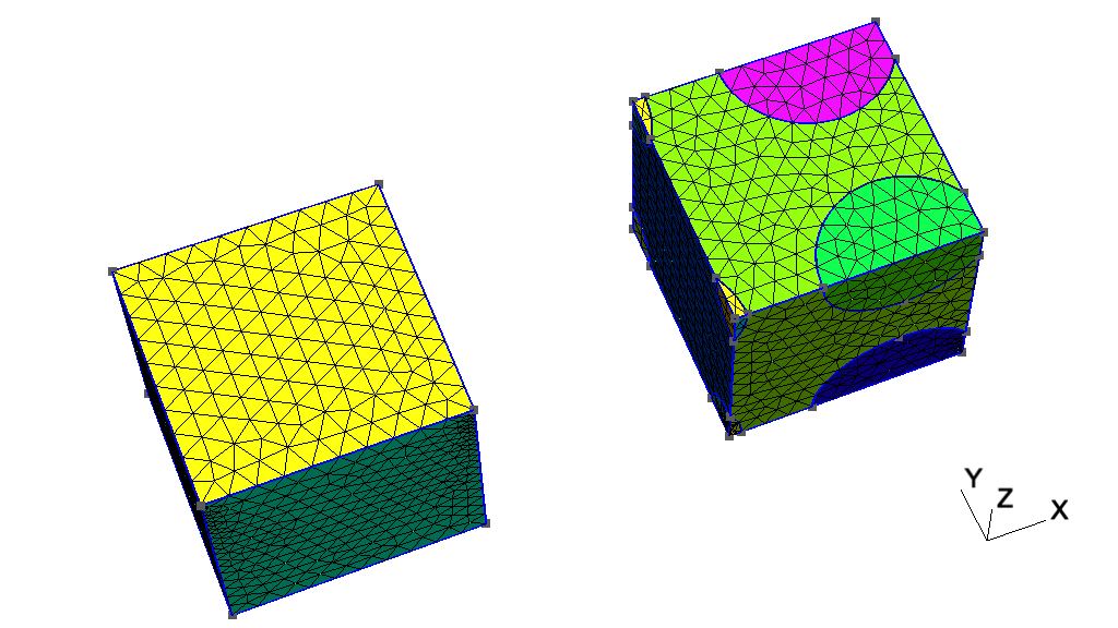
Figure 1:Meshed SG. This example uses the model on the right with particle inclusions only. Source: Gmsh tutorial 18.
Material Properties
Matrix
Density: 1000 kg/m3
Young’s Modulus: 1.0e9 Pa
Poisson’s Ratio: 0.3
Inclusion
Density: 2500 kg/m3
Young’s Modulus: 1.0e11 Pa
Poisson’s Ratio: 0.25
File Structure
gmsh_t18/
├── README.md              # This documentation
├── run.py                 # Main parametric study script
├── build_sg.py            # Gmsh geometry generation
├── convert.py             # Format conversion (Gmsh → SwiftComp)
├── visualization.ipynb    # Result visualizations
├── data/                  # Input files
│   └── materials.json       # Material property definitions
└── results/               # Output files
    └── t18_results.csv      # Analysis results
Running the Analysis
Execute the complete parametric study:
# Install only this example's dependencies
cd examples/gmsh_t18
uv sync

# Run the parametric study in the example environment
uv run python run.py

# Results saved to results/t18_results.csv
# Individual case files in evals/ directory
If you want the notebook visualization dependencies as well:
uv sync --extra notebookAnalysis Workflow Scripting
In general, the analysis workflow consists of the following steps:
Geometry generation with Gmsh
Format conversion to SwiftComp
Running the parametric study
Geometry Generation with Gmsh
The SG geometry is created using the Gmsh Python API in build_sg.py based on the official script t18.py.
The script is modified in the following ways:
Setting periodicity is converted to a function and applied to all three pairs of faces.
Add physical groups for matrix and inclusion volumes to store material assignments.
1 2 3 4 5 6 7 8 9 10 11 12 13 14 15 16 17 18 19 20 21 22 23 24 25 26 27 28 29 30 31 32 33 34 35 36 37 38 39 40 41 42 43 44 45 46 47 48 49 50 51 52 53 54 55 56 57 58 59 60 61 62 63 64 65 66 67 68 69 70 71 72 73 74 75 76 77 78 79 80 81 82 83 84 85 86 87 88 89 90 91 92 93 94 95 96 97 98 99 100 101 102 103 104 105 106 107 108 109 110 111 112 113 114 115 116 117 118 119 120 121 122 123 124 125 126 127 128 129 130 131 132 133 134 135 136 137 138 139 140 141 142 143 144 145 146 147 148 149 150 151 152 153 154 155 156 157 158 159 160 161 162 163 164 165 166 167 168 169 170 171 172 173 174 175 176 177 178 179 180 181 182 183 184 185 186 187 188 189 190 191 192 193 194 195 196 197 198 199 200 201 202 203 204 205 206 207 208 209 210 211 212 213 214 215 216 217 218 219 220 221 222 223 224 225 226 227 228 229 230 231 232 233 234 235 236 237 238# ------------------------------------------------------------------------------ # # Gmsh Python tutorial 18 # # Periodic meshes # # ------------------------------------------------------------------------------ # Periodic meshing constraints can be imposed on surfaces and curves. import gmsh # import math import os import sys import json eps = 1e-3 def set_periodic_faces(min_bbox, max_bbox, translation): """ Set periodicity between two faces based on bounding boxes. Args: min_bbox: Bounding box for the minimum face (xmin, ymin, zmin, xmax, ymax, zmax) max_bbox: Bounding box for the maximum face (xmin, ymin, zmin, xmax, ymax, zmax) translation: 4x4 affine transformation matrix """ # Get all surfaces on the minimum side min_faces = gmsh.model.getEntitiesInBoundingBox(min_bbox[0], min_bbox[1], min_bbox[2], min_bbox[3], min_bbox[4], min_bbox[5], 2) for i in min_faces: # Get the bounding box of each minimum surface xmin, ymin, zmin, xmax, ymax, zmax = gmsh.model.getBoundingBox(i[0], i[1]) # Translate the bounding box and look for surfaces inside it max_faces = gmsh.model.getEntitiesInBoundingBox(max_bbox[0], max_bbox[1], max_bbox[2], max_bbox[3], max_bbox[4], max_bbox[5], 2) # For all the matches, compare the corresponding bounding boxes for j in max_faces: xmin2, ymin2, zmin2, xmax2, ymax2, zmax2 = gmsh.model.getBoundingBox(j[0], j[1]) # Apply inverse translation to compare if translation[3] != 0: # x-translation xmin2 -= translation[3] xmax2 -= translation[3] if translation[7] != 0: # y-translation ymin2 -= translation[7] ymax2 -= translation[7] if translation[11] != 0: # z-translation zmin2 -= translation[11] zmax2 -= translation[11] # If bounding boxes match, apply the periodicity constraint if (abs(xmin2 - xmin) < eps and abs(xmax2 - xmax) < eps and abs(ymin2 - ymin) < eps and abs(ymax2 - ymax) < eps and abs(zmin2 - zmin) < eps and abs(zmax2 - zmax) < eps): gmsh.model.mesh.setPeriodic(2, [j[1]], [i[1]], translation) def build_sg( radius=0.35, fn_sg_base='sg', fn_materials='materials.json', mesh_size=0.1, nopopup=False ): # Load materials from JSON file with open(fn_materials, 'r') as f: materials_data = json.load(f) # Create a mapping from material name to material ID material_name_to_id = {} for material in materials_data: material_name_to_id[material['name']] = material['id'] # Get material IDs for matrix and inclusion MATRIX_ID = material_name_to_id['matrix'] INCLUSION_ID = material_name_to_id['inclusion'] gmsh.initialize() gmsh.model.add("sg") # For more complicated cases, finding the corresponding surfaces by hand can # be tedious, especially when geometries are created through solid # modelling. Let's construct a slightly more complicated geometry. # We start with a cube and some spheres: gmsh.model.occ.addBox(2, 0, 0, 1, 1, 1, 10) x = 2 - 0.3 y = 0 z = 0 gmsh.model.occ.addSphere(x, y, z, radius, 11) gmsh.model.occ.addSphere(x + 1, y, z, radius, 12) gmsh.model.occ.addSphere(x, y + 1, z, radius, 13) gmsh.model.occ.addSphere(x, y, z + 1, radius, 14) gmsh.model.occ.addSphere(x + 1, y + 1, z, radius, 15) gmsh.model.occ.addSphere(x, y + 1, z + 1, radius, 16) gmsh.model.occ.addSphere(x + 1, y, z + 1, radius, 17) gmsh.model.occ.addSphere(x + 1, y + 1, z + 1, radius, 18) # We first fragment all the volumes, which will leave parts of spheres # protruding outside the cube: out, outmap = gmsh.model.occ.fragment([(3, 10)], [(3, i) for i in range(11, 19)]) gmsh.model.occ.synchronize() # Track which volumes came from the box (matrix) and which from spheres (inclusions) # outmap[i] contains the list of volumes that resulted from fragmenting entity i # Index 0 corresponds to the box (tag 10), indices 1-8 correspond to spheres (tags 11-18) matrix_volumes = [] inclusion_volumes = [] # Get volumes from the box (matrix material) if len(outmap) > 0 and len(outmap[0]) > 0: for dim_tag in outmap[0]: if dim_tag[0] == 3: # Only 3D volumes matrix_volumes.append(dim_tag[1]) # Get volumes from the spheres (inclusion material) for i in range(1, min(9, len(outmap))): if len(outmap[i]) > 0: for dim_tag in outmap[i]: if dim_tag[0] == 3: # Only 3D volumes inclusion_volumes.append(dim_tag[1]) # Ask OpenCASCADE to compute more accurate bounding boxes of entities using # the STL mesh: gmsh.option.setNumber("Geometry.OCCBoundsUseStl", 1) # We then retrieve all the volumes in the bounding box of the original cube, # and delete all the parts outside it: vin = gmsh.model.getEntitiesInBoundingBox(2 - eps, -eps, -eps, 2 + 1 + eps, 1 + eps, 1 + eps, 3) for v in vin: out.remove(v) gmsh.model.removeEntities(out, True) # Delete outside parts recursively # Update the volume lists to only include volumes inside the bounding box vin_tags = [v[1] for v in vin] inclusion_volumes = [v for v in inclusion_volumes if v in vin_tags] matrix_volumes = [v for v in matrix_volumes if (v in vin_tags and v not in inclusion_volumes)] # We now set a non-uniform mesh size constraint (again to check results # visually): p = gmsh.model.getBoundary(vin, False, False, True) # Get all points gmsh.model.mesh.setSize(p, mesh_size) p = gmsh.model.getEntitiesInBoundingBox(2 - eps, -eps, -eps, 2 + eps, eps, eps, 0) gmsh.model.mesh.setSize(p, mesh_size) # --------------- # Set Periodicity # --------------- # x-faces # To impose that the mesh on surface 2 (the right side of the cube) should # match the mesh from surface 1 (the left side), the following periodicity # constraint is set: # The periodicity transform is provided as a 4x4 affine transformation matrix, # given by row. translation = [ 1, 0, 0, 1, 0, 1, 0, 0, 0, 0, 1, 0, 0, 0, 0, 1 ] # During mesh generation, the mesh on surface 2 will be created by copying # the mesh from surface 1. # We now identify corresponding surfaces on the left and right sides of the # geometry automatically using the helper function. xmin_bbox = (2 - eps, -eps, -eps, 2 + eps, 1 + eps, 1 + eps) xmax_bbox = (2 - eps + 1, -eps, -eps, 2 + eps + 1, 1 + eps, 1 + eps) set_periodic_faces(xmin_bbox, xmax_bbox, translation) # y-faces translation = [ 1, 0, 0, 0, 0, 1, 0, 1, 0, 0, 1, 0, 0, 0, 0, 1 ] # Set periodicity for y-faces using the helper function ymin_bbox = (2 - eps, -eps, -eps, 2 + eps + 1, eps, eps + 1) ymax_bbox = (2 - eps, -eps + 1, -eps, 2 + eps + 1, eps + 1, eps + 1) set_periodic_faces(ymin_bbox, ymax_bbox, translation) # z-faces translation = [ 1, 0, 0, 0, 0, 1, 0, 0, 0, 0, 1, 1, 0, 0, 0, 1 ] # Set periodicity for z-faces using the helper function zmin_bbox = (2 - eps, -eps + 1, -eps, 2 + eps + 1, eps + 1, eps) zmax_bbox = (2 - eps, -eps + 1, -eps + 1, 2 + eps + 1, eps + 1, eps + 1) set_periodic_faces(zmin_bbox, zmax_bbox, translation) gmsh.model.mesh.generate(3) # Assign material IDs to elements based on which volume they belong to # Use material IDs from materials.json # Create physical groups for matrix and inclusion materials print(f'{matrix_volumes=}') if len(matrix_volumes) > 0: gmsh.model.addPhysicalGroup(3, matrix_volumes, MATRIX_ID) gmsh.model.setPhysicalName(3, MATRIX_ID, "matrix") print(f'{inclusion_volumes=}') if len(inclusion_volumes) > 0: gmsh.model.addPhysicalGroup(3, inclusion_volumes, INCLUSION_ID) gmsh.model.setPhysicalName(3, INCLUSION_ID, "inclusion") # Write the mesh file first gmsh.write(f"{fn_sg_base}.msh") # Launch the GUI to see the results: if not nopopup: gmsh.fltk.run() gmsh.finalize() if __name__ == "__main__": build_sg()
Structure genome generation using Gmsh Python API
Format Conversion
The convert.py script handles the format conversion from Gmsh to SwiftComp. The overall steps are straightforward and as follows:
Read the Gmsh mesh file
Add materials to the model
Write the SwiftComp model to file
1 2 3 4 5 6 7 8 9 10 11 12 13 14 15 16 17 18 19 20 21import os import sgio def convert_sg( fn_sg_in='sg.msh', fn_materials='materials.json', fn_sg_out='sg.sg' ): sg = sgio.read(fn_sg_in, file_format='gmsh') # Load materials from JSON file script_dir = os.path.dirname(os.path.abspath(__file__)) materials_file = os.path.join(script_dir, fn_materials) sg.materials = sgio.read_materials_from_json(materials_file) sgio.write(sg, fn_sg_out, file_format='sc') if __name__ == "__main__": convert_sg()
Converting Gmsh mesh to SwiftComp format
Main Parametric Study
The parametric study sweeps through inclusion radii and computes effective properties for each case. Implementation in run.py:
1 2 3 4 5 6 7 8 9 10 11 12 13 14 15 16 17 18 19 20 21 22 23 24 25 26 27 28 29 30 31 32 33 34 35 36 37 38 39 40 41 42 43 44 45 46 47 48 49 50 51 52 53 54 55 56 57 58 59 60 61import logging logger = logging.getLogger(__name__) logger.setLevel(logging.INFO) fh = logging.FileHandler('run.log') fh.setLevel(logging.INFO) logger.addHandler(fh) import os import numpy as np import pandas as pd import sgio from build_sg import build_sg from convert import convert_sg working_dir = 'evals' # Run SG analysis for a range of radii radii = np.linspace(0.1, 0.4, 7) logger.info(f'{radii=}') out = [] eng_const_names = [ 'e1', 'e2', 'e3', 'nu12', 'nu13', 'nu23', 'g12', 'g13', 'g23' ] for i, radius in enumerate(radii): logger.info(f'Running for radius: {radius}') _out = {'radius': radius} # Create working directory if it doesn't exist wd = os.path.join(working_dir, f'eval.{i}') if not os.path.exists(wd): os.makedirs(wd) # Build SG using gmsh fn_sg_base = os.path.join(wd, 'sg') build_sg(radius=radius, fn_sg_base=fn_sg_base, fn_materials='data/materials.json', mesh_size=0.05, nopopup=True) # Convert to SwiftComp format fn_sg_sc = f'{fn_sg_base}.sg' convert_sg(fn_sg_in=f'{fn_sg_base}.msh', fn_sg_out=fn_sg_sc) _out['fn_sg_sc'] = fn_sg_sc # Run SwiftComp and read output sgio.run('swiftcomp', fn_sg_sc, 'h', smdim=3) sc_out = sgio.read_output_model(f'{fn_sg_sc}.k', file_format='sc', model_type='sd1') _props = sc_out.model_dump(exclude_none=True) for i, name in enumerate(eng_const_names): _out[name] = _props[name] out.append(_out) # Write results to CSV df = pd.DataFrame(out) df.to_csv('results/t18_results.csv', index=False)
Main parametric study loop
Results and Visualization
The results are saved to results/t18_results.csv and can be visualized using the Jupyter notebook Gmsh Python tutorial 18.
import pandas as pd
import plotly.graph_objects as go
from plotly.subplots import make_subplots

eng_const_names = [
    'e1', 'e2', 'e3', 'nu12', 'nu13', 'nu23', 'g12', 'g13', 'g23'
    ]
eng_const_labels = [
    r'$E_1$', r'$E_2$', r'$E_3$',
    r'$\nu_{12}$', r'$\nu_{13}$', r'$\nu_{23}$',
    r'$G_{12}$', r'$G_{13}$', r'$G_{23}$'
    ]

df = pd.read_csv('results/t18_results.csv')

# Create 3x3 subplot grid
fig = make_subplots(
    rows=3, cols=3,
    subplot_titles=eng_const_labels,
    shared_xaxes=True,
    shared_yaxes='rows',
    vertical_spacing=0.1,
    horizontal_spacing=0.05
)

# Plot each engineering constant
for i, const_name in enumerate(eng_const_names):
    row = i // 3 + 1
    col = i % 3 + 1

    fig.add_trace(
        go.Scatter(
            x=df['radius'],
            y=df[const_name],
            mode='lines+markers',
            line=dict(width=2, color='black'),
            name=eng_const_labels[i],
            showlegend=False
        ),
        row=row, col=col
    )

# Update layout
fig.update_layout(
    title="Engineering Constants vs Radius",
    template='plotly_white',
    height=600,
    width=600,
)

# Update axes labels
fig.update_xaxes(title_text="Radius", row=3, col=1)
fig.update_xaxes(title_text="Radius", row=3, col=2)
fig.update_xaxes(title_text="Radius", row=3, col=3)

fig.update_yaxes(title_text="Young's Modulus (Pa)", row=1, col=1)
fig.update_yaxes(title_text="Poisson's Ratio", row=2, col=1)
fig.update_yaxes(title_text="Shear Modulus (Pa)", row=3, col=1)


fig.show()Engineering constants vs fiber radius for the T18 example.